ggplot(mtcars, aes(x = as.factor(cyl), fill = as.factor(cyl) )) +
  geom_bar( ) +
  scale_fill_manual(values = flex(c("cyan", "red", "blue"),
                                  c(200, 400, 600)) ) +
  theme(legend.position = "none")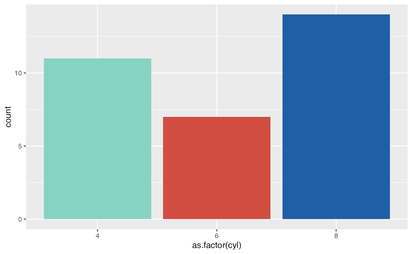
ggplot(mtcars, aes(x = as.factor(cyl), fill = as.factor(cyl) )) +
  geom_bar( ) +
  scale_fill_manual(values = flex(c("cyan", "red", "blue"), 500) ) +
  theme(legend.position = "none")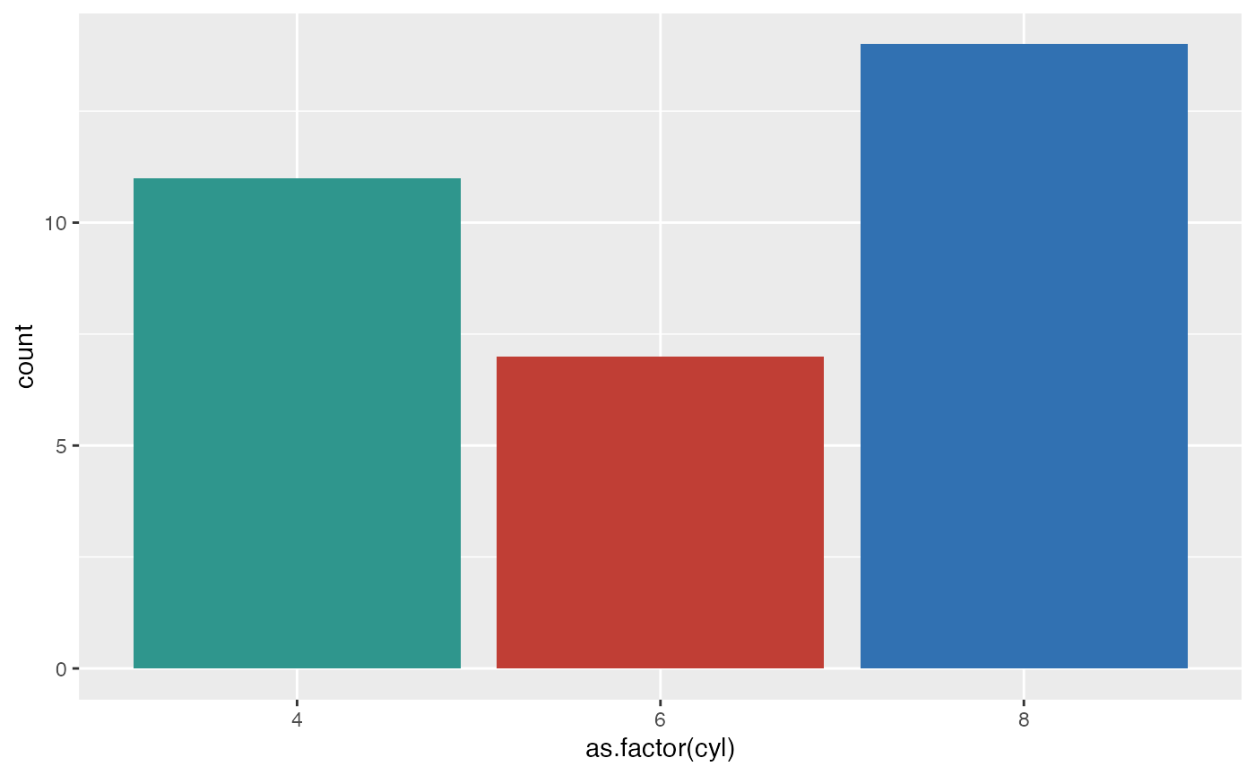
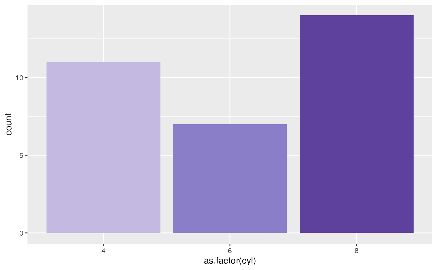
ggplot(mtcars, aes(x = as.factor(cyl), fill = as.factor(cyl) )) +
  geom_bar( ) +
  scale_fill_manual(values = flex("purple", c(200, 400, 600)) ) +
  theme(legend.position = "none")